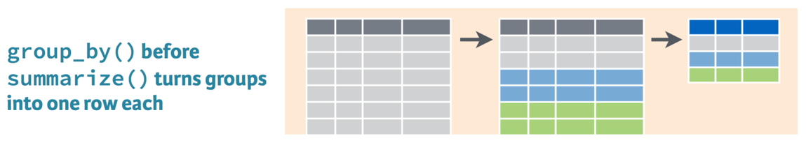
Group by
The group_by verb
In the last lesson, you used the summarize verb to calculate an average either,
- across all countries (the entire dataset)
- within a particular country (filtered data)
In this lesson you'll learn the group_by verb, which opens up a new option for calculating an average:
- within each country
The group_by verb
The summarize verb
(music_top200
  >> filter(_.country == "Japan")
>> summarize(avg_duration = _.duration.mean()))| avg_duration | |
|---|---|
| 0 | 250.53499 |
Summarizing by country
(music_top200
  >> group_by(_.country)
  >> summarize(avg_duration = _.duration.mean())
)| country | avg_duration | |
|---|---|---|
| 0 | Argentina | 212.847855 |
| 1 | Australia | 204.795300 |
| 2 | Austria | 184.894870 |
| ... | ... | ... |
| 59 | United States | 190.827500 |
| 60 | Uruguay | 210.796985 |
| 61 | Viet Nam | 217.222830 |
62 rows × 2 columns
Summarizing by continent and position
(music_top200
  >> group_by(_.continent, _.position)
  >> summarize(
      min_streams = _.streams.min(),
      max_streams = _.streams.max()
  )
)| continent | position | min_streams | max_streams | |
|---|---|---|---|---|
| 0 | Africa | 1 | 94422 | 94422 |
| 1 | Africa | 2 | 74689 | 74689 |
| 2 | Africa | 3 | 67552 | 67552 |
| ... | ... | ... | ... | ... |
| 997 | Oceania | 198 | 44570 | 225951 |
| 998 | Oceania | 199 | 44364 | 225492 |
| 999 | Oceania | 200 | 44291 | 225179 |
1000 rows × 4 columns
Summarizing by continent and position
(music_top200

  >> summarize(
      min_streams = _.streams.min(),
      max_streams = _.streams.max()
  )
)| min_streams | max_streams | |
|---|---|---|
| 0 | 1470 | 12987027 |
Summarizing by continent and position
(music_top200
  >> filter(_.continent == "Oceania", _.position == 1)
  >> summarize(
      min_streams = _.streams.min(),
      max_streams = _.streams.max()
  )
)| min_streams | max_streams | |
|---|---|---|
| 0 | 321272 | 1757343 |
Summarizing by continent and position
(music_top200
  >> group_by(_.continent, _.position)
  >> summarize(
      min_streams = _.streams.min(),
      max_streams = _.streams.max()
  )
)| continent | position | min_streams | max_streams | |
|---|---|---|---|---|
| 0 | Africa | 1 | 94422 | 94422 |
| 1 | Africa | 2 | 74689 | 74689 |
| 2 | Africa | 3 | 67552 | 67552 |
| ... | ... | ... | ... | ... |
| 997 | Oceania | 198 | 44570 | 225951 |
| 998 | Oceania | 199 | 44364 | 225492 |
| 999 | Oceania | 200 | 44291 | 225179 |
1000 rows × 4 columns
Let's practice!
Exercise 1:
Modify the code below so it calculates max popularity and average danceability for each artist.
| max_popularity | avg_danceability | |
|---|---|---|
| 0 | 99 | 0.677937 |
1 rows × 2 columns
Make a scatterplot of the data.
In the plot above, what strange thing is going on with the distribution of max popularity?
possible answer
There are many artists with a max popularity of 0!
Exercise 2:
In the last exercise of the facets chapter, you examined track features for three artists.
We used a plot and intuition to judge who tended to have highest energy and valence tracks.
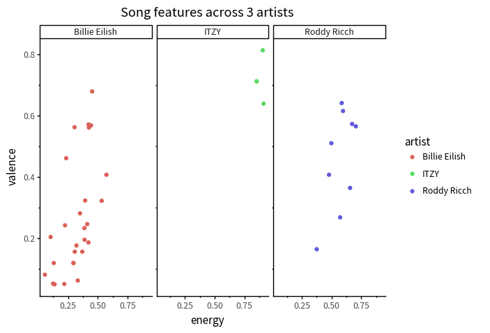
Now you should be able to answer the question more directly!
Use a grouped summarize to calculate the mean energy and valence for each artist.
Q: In this data, which artist has the lowest average energy, and what is its value?
answer
Billie Eilish, 0.321004Q: What about for lowest average valence?